Dynamic Models (Continuous Time)

In this post, I look at continuous time models. Price dynamics are described and wealth dynamics are derived. I then look at dynamic programming, describing the Hamilton Jacobi Bellman partial differential equation. I apply this to the case of constant investment opportunities and CRRA utility (including log utility). The results described in discrete time are shown to hold here as well. I then look at cases where investment opportunities fluctuate, reflecting the dynamics of a scalar Markovian process. In the first example, the driving variable is the (stochastic) cash rate. This model allows to discuss the role of bonds as hedging instruments within portfolios. In the second example, the cash rate is constant but the equity premium fluctuates and the equity index is more volatile in the short term than in the long term. This makes the optimal equity weight dependent on the investment horizon.

---

Why continuous time?

• Decisions are taken at specific instants which are themselves decision variables. The underlying time scale is continuous. Realism therefore suggests exploring continuous time.

• Continuous time leads to some simplifications. Discrete time mathematics are harder than it looks. As an example, continuous time calculus often provides closed form expressions where discrete time does not.

  • Example of a simplification: log normal markets

• However: to properly ground continuous time processes requires heavy machinary; the Ito integral is only about \(60\) years old. See summary on stochastic calculus.

Price dynamics and total return processes (1)

• Geometric SDEs and particularly the GBM are good candidates to model equity price processes. Equity processes however distribute dividends. The dividends need to be integrated to judge the attractiveness of the investment.

• The ex-dividend rate of return is: \[\frac{dP_{t}}{P_{t}}.\]

• If a contract distributes dividends \(\delta_{t}dt\) in a time interval of size \(dt\), the total rate of return of a contract is: \[\frac{dP_{t}+\delta_{t}dt}{P_{t}}.\]

Price dynamics and total return processes (2)

• If I own \(n_{t}\) equity contracts at date \(t\), I get the total return computed above. Yet, at \(t+dt\), I have cash to invest. I purchase \(dn_{t}\) shares: \[dn_{t}P_{t}=n_{t}\delta_{t}dt,\] \[\frac{dn_{t}}{n_{t}}=\frac{\delta_{t}}{P_{t}}dt.\]

• The number of shares grows at a rate given by the dividend yield. It’s a finite variation process.

• A total rate of return index is a portfolio with an investment policy! Its value \(n_{t}P_{t}\) grows at a rate: \[\frac{d(n_{t}P_{t})}{n_{t}P_{t}}=\frac{n_{t}dP_{t}}{n_{t}P_{t}}+\frac{P_{t}dn_{t}}{n_{t}P_{t}}=\frac{dP_{t}+\delta_{t}dt}{P_{t}}.\]

The cash account

• If some money is put on a cash account and left alone, it accumulates at a rate that is predetermined: \[\frac{dD_{t}}{D_{t}}=r^{f}_{t}dt,\] or in integral from: \[D_{t}-D_{s}=\int_{s}^{t}D_{u}r^{f}_{u}du.\]

• However, the above integral \(\int_{s}^{t}D_{u}r^{f}_{u}du\) also measures the gain attached to having \(D_{u}\) on the cash account between date \(s\) and date \(t\), regardless of whether money is added or redeemed from the cash account in this time interval.

Wealth dynamics (1)

• We now consider a set of securities indexed by \(i\in \{1,2,\ldots,N\}\), with price processes \((P_{i,t})_{t\in \mathbb{R}_{+}}\) that are semimartingales and follow geometric diffusions: \[\frac{dP_{i,t}}{P_{i,t}}=\mu_{i,t}dt+\sigma_{i,t}dB_{t}.\]

• Dimensions:

  • \(B_{t}\) is a \((N,1)\) multivariate Brownian motion with independent components
  • accordingly \(\sigma_{i,t}\) is a \((1,N)\) volatility matrix

• As usual, when a cash account is present, it receives index \(0\). The set of instruments is denoted \(\cal{I}\) as usual.

• In this case, it is convenient to introduce excess returns: \[\frac{dP_{i,t}}{P_{i,t}}=r^{f}_{t}dt+(\mu_{i,t}-r^{f}_{t})dt+\sigma_{i,t}dB_{t}.\]

Wealth dynamics (2)

• The gain generated by holding \(n_{i,u}\) units of security \(i\) is: \[G_{i,t}-G_{i,s}=\int_{s}^{t}n_{i,u}dP_{i,u}.\]

• Assume positions \(n_{i,u}\) on risky securities are held. The gain made thereby over a time interval \([s,t]\) is: \[\hat{G}_{t}-\hat{G}_{s}=\sum_{i=1}^{N}\int_{s}^{t}n_{i,u}dP_{i,u}.\]

• The total gain made over cash and risky securities is thus: \[W_{t}-W_{s}=\int_{s}^{t}D_{u}r^{f}_{u}du+\sum_{i=1}^{N}\int_{s}^{t}n_{i,u}dP_{i,u}.\]

Wealth dynamics (3)

• Assume now that we are at a trading date. Barring transaction costs, trading does not change the value of the portfolio. We therefore should have at all times that the value of the portfolio only changes as a result of the gains made on the securities, i.e.: \[dW_{u}=dD_{u}+\sum_{i=1}^{N}n_{i,u}dP_{i,u}.\]

• This equation is called the self financing condition. It is really the counterpart of \(W_{t+1}=W_{t}(\pi_{t}'R_{t+1})\) in discrete time.

• We can rewrite this as: \[\frac{dW_{u}}{W_{u}}=\frac{D_{u}}{W_{u}}\frac{dD_{u}}{D_{u}}+\sum_{i=1}^{N}\frac{n_{i,u}P_{i,u}}{W_{u}}\frac{dP_{i,u}}{P_{i,u}}.\]

• We can finally introduce the portfolio shares \((\pi_{i,t})_{i\in {\cal I}}\): \[\frac{dW_{u}}{W_{u}}=\pi_{0,u}r^{f}_{u}du+\sum_{i=1}^{N}\pi_{i,u}(\mu_{i,u}du+\sigma_{i,u}dB_{u}),\] where we have used the fact that at any time: \[W_{t}=D_{t}+\sum_{i=1}^{N}n_{i,u}P_{i,u},\] i.e.: \[\sum_{i\in{\cal I}} \pi_{i,u}=1.\]

Wealth dynamics (4)

• We now need more compact notations.

• We write the dynamics of securities prices in vector notations: \[\frac{dP_{t}}{P_{t}}=\mu_{t}dt+\sigma_{t}dB_{t},\] with (abuse!) the left hand side denoting the vector of instantaneous rates of returns.

• Dimensions:

  • \(\mu_{t}\) is \((N,1)\)
  • \(\sigma_{t}\) is \((N,N)\)

• In the very short term, risk is driven by the term \(\sigma_{t}dB_{t}\). Thus the short term covariance matrix of \(dP_{t}/P_{t}\) (rates of return) is¹: \[\text{Var}_{t}[\frac{dP_{t}}{P_{t}}]=E_{t}[\sigma_{t}dB_{t}dB_{t}'\sigma_{t}'].\]

• The covariance matrix (size \((N,N)\)) of securities is thus: \[\Sigma_{t}=\sigma_{t}\sigma_{t}'.\] It should be thought of as annualized.

Wealth dynamics (5)

• The vector \(\pi_{t}\) (size \((N,1)\)) represents the set of weights on risky assets.

• The scalar \(\pi_{0,t}\) represents the weight on the riskless asset.

• We can write the wealth dynamics as: \[\frac{dW_{u}}{W_{u}}=(\pi_{0,u}r^{f}_{u}+\pi_{u}'\mu_{u})du+\pi_{u}'\sigma_{u}dB_{u},\] or: \[\frac{dW_{u}}{W_{u}}=r^{f}_{u}du+\pi_{u}'(\mu_{u}-r^{f}_{u}\pmb{e})du+\pi_{u}'\sigma_{u}dB_{u}.\]

• This geometric equation implies: \[ W_{t}=W_{0}\exp\Big(\int_{0}^{t}r^{f}_{u}du+\int_{0}^{t}\pi_{u}'(\mu_{u}-r^{f}_{u}\pmb{e})du- \\ \frac{1}{2}\int_{0}^{t}\pi_{u}'\Sigma_{u}\pi_{u}du+\int_{0}^{t}\pi_{u}'\sigma_{u}dB_{u}\Big). \]

• When all coefficients (\(\mu_{u}\),\(\Sigma_{u}\),\(r^{f}_{u}\),\(\pi_{u}\)) are deterministic, wealth follows a log normal process. Log-normal models are not available in discrete time (the sum of two log normal variables is not log-normal).

Wealth dynamics (6)

• In the presence of income \(Y_{t}dt\) and consumption \(C_{t}dt\) per unit of time, the dynamic of wealth is: \[\frac{dW_{u}}{W_{u}}=r^{f}_{u}+\pi_{u}'(\mu_{u}-r^{f}_{u}\pmb{e})du+\pi_{u}'\sigma_{u}dB_{u}+y_{u}du-c_{u}du,\] with \(c_{u}=C_{u}/W_{u}\) and \(y_{u}=Y_{u}/W_{u}\).

Absence of arbitrage

• One version of Farkas’s Lemma says that on finite dimensional vector spaces, if the kernel of a set of linear forms \((f_{i})_{1\le i \le P}\) is included in that of a linear form \(g\), then \(g\) is a linear combination of the \(f_{i}\)s: \[g=\sum_{i=1}^{P}\lambda_{i}f_{i}.\]

• As an application, suppose that the absence of any exposure to the sources of risk (\(\sigma' \pi=0_{N}\)) implies that the excess return is zero (\((\mu-r^{f}e)'\pi=0\)), then: \[\mu-r^{f}e=\sigma\lambda.\]

• Here, the columns of \(\sigma\) give the family of linear of forms \((f_{i})_{1\le i \le N}\) while the excess return is \(g\).

• The premise says that ‘no risk implies no excess return’, and the conclusion says that risky asset’s excess return are proportional to risk exposure. The vector \(\lambda\) is the vector of risk prices.

Remarks

• If the distribution of wealth is log-normal, one can easily compute expected utility of wealth for CRRA utility functions.

• Indeed: \[E[\frac{W^{1-\gamma}}{1-\gamma}]=\frac{1}{1-\gamma}E\left[\exp\left((1-\gamma)\log(W)\right)\right]=\] \[\frac{1}{1-\gamma}\exp\left((1-\gamma)E[\log(W)]+\frac{1}{2}(1-\gamma)^{2}\text{Var}\left(\log(W)\right)\right).\]

• This allows to make explicit calculations in log-normal markets.

Investment opportunities

• The data describing investment opportunities are \((r^{f}_{u},\mu_{u},\sigma_{u})\).

• Investment opportunities are constant if the data do not depend on time.

• Alternatively I will assume that all data depend on a scalar Markovian state process \((x_{t})_{t\in \mathbb{R}_{+}}\) with dynamics described by a diffusion: \[dx_{t}=\phi_{t}dt+\nu_{t}dB_{t},\] where \(\nu_{t}\) is of size \((1,N)\).

• I describe dynamic programming in this context.

Dynamic programming (1)

• We will consider the following optimization problem (consumption but no income): \[V(t,x_{t},W_{t})=\] \[\underset{(\pi_{[t,T]},C_{[t,T]})}{\text{max}} \; E_{t}\Big[\int_{t}^{T} e^{-\delta(u-t)}u(C_{u})du+ \;e^{-\delta(T-t)}U(W_{T})\Big]\] \[\text{s.t.}\] \[\; \frac{dW_{u}}{W_{u}}=r^{f}_{u}du+\pi_{u}'(\mu(x_{u})-r^{f}(x_{u}))du+\pi_{u}'\sigma(x_{u})dB_{u}-c_{u}du\] \[\; c_{u} \geq 0\] \[\; W_{u} > 0.\]

• \(V_{t}\) is discounted back at time \(t\), not at time \(0\).

Dynamic programming (2)

• I heuristically derive the Hamilton Jacobi Bellman equation, a partial differential equation.

• We have: \[V(t,x_{t},W_{t})=\] \[\underset{(\pi_{t},C_{t})}{\text{max}}\Big\{u(C_{t})\Delta t+ e^{-\delta \Delta t}E_{t}[V(t+\Delta t,x_{t+\Delta t},W_{t+\Delta t})]\Big\}.\]

Dynamic programming (3)

• We transform this multiplying the whole equation by \(e^{\delta \Delta t}\), then subtracting \(V(t,x_{t},W_{t})\), and finally, dividing by \(\Delta t\):

\[ \frac{e^{\delta \Delta t}-1}{\Delta t}V(t,x_{t},W_{t})= \underset{(\pi_{t},C_{t})}{\text{max}}\Big\{e^{\delta \Delta t}u(C_{t})+\] \[\frac{1}{\Delta t}E_{t}[V(t+\Delta t,x_{t+\Delta t},W_{t+\Delta t})-V(t,x_{t},W_{t})]\Big\}. \]

Dynamic programming (4)

• We now take the limit as \(\Delta t\) goes to zero.

• \(\frac{e^{\delta \Delta t}-1}{\Delta t}\) converges to the derivative of \(\exp(\delta x)\) at \(x=0\), i.e. \(\delta\).

• Ito’s formula is then used to express the expectation term on the right hand side, leading to the following expression: \[\lim_{\Delta t \rightarrow 0}E_{t}[\frac{1}{\Delta t}\left(V(t+\Delta t,x_{t+\Delta t},W_{t+\Delta t})-V(t,x_{t},W_{t})\right)]=\] \[\frac{\partial V}{\partial t}+\frac{\partial V}{\partial x}\phi+\frac{\partial V}{\partial W}W(r^{f}_{t}+ \pi_{t}'(\mu_{t}-r^{f}_{t}\pmb{e})-c_{t})+\] \[\frac{1}{2}\frac{\partial^{2} V}{\partial W^{2}}W_{t}^{2}\pi_{t}'\Sigma_{t}\pi_{t}+\frac{1}{2}\frac{\partial^{2} V}{\partial x^{2}}\nu_{t}\nu_{t}'+\frac{\partial^{2} V}{\partial W \partial x}W_{t}\pi_{t}'\sigma_{t}\nu_{t}'.\]

Dynamic programming (5)

• We get: \[0=\underset{(\pi_{t},C_{t})}{\text{max}}\Big\{ u(C_{t})-\delta V(t,x_{t},W_{t})+\] \[\frac{\partial V}{\partial t}+\frac{\partial V}{\partial x}\phi+\frac{\partial V}{\partial W}W_{t}(r^{f}_{t}+ \pi_{t}'(\mu_{t}-r^{f}_{t}\pmb{e})-c_{t})+\] \[\frac{1}{2}\frac{\partial^{2} V}{\partial W^{2}}W_{t}^{2}\pi_{t}'\Sigma_{t}\pi_{t}+\frac{1}{2}\frac{\partial^{2} V}{\partial x^{2}}\nu_{t}\nu_{t}'+\frac{\partial^{2} V}{\partial W \partial x}W_{t}\pi_{t}'\sigma_{t}\nu_{t}'\Big\}.\]

• This partial differential equation is called the Hamilton Jacobi Bellman equation.

Dynamic programming (5)

• Consumption si given by (envelope condition): \[u'(C_{t})=\frac{\partial V}{\partial W}.\]

• To determine the portfolio positions, we look at the terms in HJB which involve \(\pi_{t}\). They determine a quadratic form with leading term: \[\frac{1}{2}\frac{\partial^{2} V}{\partial W^{2}}W_{t}^{2}\pi_{t}'\Sigma_{t}\pi_{t}.\]

• In the cases that we will explore, the value function is concave. It’s second derivative is negative and the quadratic form is negative definite (as \(\Sigma_{t}\) is positive definite). The portfolio positions are tied to the partial derivatives of the value function through the first order condition which reads: \[\frac{\partial V}{\partial W}W_{t}(\mu_{t}-r^{f}_{t}\pmb{e})+ \frac{\partial^{2} V}{\partial W^{2}}W_{t}^{2}\Sigma_{t}\pi_{t}^{\star}+\frac{\partial^{2} V}{\partial W \partial x}W_{t}\sigma_{t}\nu_{t}'=0.\]

• From which we get: \[\pi^{\star}_{t}=-\frac{V_{W}}{W_{t}V_{WW}}\left(\Sigma^{-1}(\mu_{t}-r^{f}_{t}\pmb{e})+\frac{V_{Wx}}{V_{W}}\Sigma^{-1}\sigma_{t}\nu_{t}'\right),\] using simplified notations for partial derivatives.

Remarks

• The optimal controls can be injected back into HJB to deliver a non linear partial differential equation.

• We have determined a partial differential equation (PDE) which the value function should obey, but we have not solved for the value function.

• Had we found a value function solution to HJB, one would need to prove that it is truly the value function of the optimal control. After all, HJB might have several solutions! One would also need to check that the corresponding control is the optimal control. These steps are called the verification step.

• To get a sense of what the verification step does, you can check the section on dynamic programming in discrete time.

Interpretation (1)

• The case without consumption delivers the same expression for the investment policy. Of course, since the PDE contains the utility of consumption, the value function itself depends on whether we have interim consumption or not.

• The quantity \(-V_{W}/(W_{t}V_{WW})\) is the inverse of relative risk aversion. It is relative risk tolerance.

• \(\Sigma^{-1}(\mu_{t}-r^{f}_{t}\pmb{e})\) is, up to a normalizing constant, an instantaneously mean variance efficient portfolio (exercise: find the constant).

Interpretation (2)

• We have: \[\frac{V_{Wx}}{V_{W}}=\frac{d\log(V_{W})}{dx}.\] This is the logarithmic derivative of the marginal value of wealth vis-à-vis the state variable.

• If we look for the portfolio \(\pi^{h}_{t}\) which return is closest to the state variable, we shoud minimize \(\text{Var}_{t}(\pi^{h\prime}_{t}dP_{t}/P_{t}-dx_{t})\). This portfolio solves: \[\text{Cov}_{t}(\frac{dP_{t}}{P_{t}},\pi^{h\prime}\frac{dP_{t}}{P_{t}}-dx_{t})=0,\] and thus: \[\text{Cov}_{t}(\sigma_{t}dB_{t},\pi^{h\prime}_{t}\sigma_{t}dB_{t}-\nu_{t}dB_{t})=0,\] \[\sigma_{t}\sigma_{t}'\pi^{h}_{t}-\sigma_{t}\nu_{t}'=0.\] Thus: \[\pi^{h}_{t}=\Sigma_{t}^{-1}\sigma_{t}\nu_{t}'.\]

• We thus recover the structure of the second portfolio in the solution. It is the hedging portfolio. Its weight is a function of the impact of the state variable on the marginal utility of wealth.

Log utility

• In the case of log utility, the value function additively separates into a component that depends on log wealth and a component that depends on the state variable.

• In the log utility case, there is thus no hedging portfolio. One says that the solution is myopic, with the investor disregarding the future changes in the investment opportunity set.

Constant opportunities

• The data describing investment opportunities are \((r^{f},\mu,\sigma)\).

• Stock returns are log-normal.

• Regardless of the presence of intermediate consumption, the optimal portfolio solves: \[\pi^{\star}_{t}=-\frac{V_{W}}{W_{t}V_{WW}}\Sigma^{-1}(\mu-r^{f}\pmb{e}).\]

• Up to the difference between continuously compounded returns and discrete time returns, the above equation is the same as in the static problem.

• Investors care about the instantaneous risk return trade-off. The latter is characterized by the maximum available Sharpe ratio (see the section on static portfolios): \[\kappa=\sqrt{(\mu-r^{f}\pmb{e})'\Sigma^{-1}(\mu-r^{f}\pmb{e})}.\]

Constant opportunities: no intermediate consumption

• I consider the case without intermediate consumption and \(\delta=0\).

• Injecting the optimal portfolio into HJB, one gets: \[V_{t}+V_{W}W(r^{f}+\pi^{\star\prime}(\mu-r^{f}\pmb{e}))+ \frac{1}{2}V_{WW}W^{2}\pi^{\star\prime}\Sigma\pi^{\star}=0\]

• This just means that \(V(t,W_{t})\) should be a local martingale for the optimal investment policy.

• The optimal portfolio solves: \[\sigma^{'}\pi^{\star}=-\frac{V_{W}}{WV_{WW}}\sigma^{-1}(\mu-r^{f}\pmb{e}).\]

• Using this we can establish: \[V_{t}+V_{W}r^{f}W-\frac{1}{2}\frac{V_{W}^{2}}{V_{WW}}||\lambda||^{2}=0,\] where \(\lambda\) is the price of risk: \[\lambda=\sigma^{-1}(\mu-r^{f}\pmb{e}).\]

• We have \(||\lambda||^{2}=\kappa^{2}\).

• One can now solve this PDE in special cases

Constant opportunities: CRRA utility

• Assume utility of terminal wealth is \(\frac{W^{1-\gamma}}{1-\gamma}\).

• One can prove that the value function is homogenous of degree \(1-\gamma\) (with our without intermediate consumption!). One can postulate: \[V(t,W)=\frac{g(t)^{\gamma}W^{1-\gamma}}{1-\gamma}.\]

• Homogeneity alone determines relative tolerance: \[-\frac{V_{W}}{W_{t}V_{WW}}=\frac{1}{\gamma},\] and thus how much of the tangent portfolio is bought: \[\pi^{\star}_{t}=\frac{1}{\gamma}\Sigma^{-1}(\mu-r^{f}\pmb{e}).\]

• The differential equation is for \(g\) is: \[(-r^{f}-\frac{1}{2}||\lambda||^{2})g(t)-\frac{\gamma}{1-\gamma}g'(t)=0.\]

• In the end: \[g(t)=\exp(-\alpha(T-t)),\] with: \[\alpha=\frac{\gamma-1}{\gamma}\left(r^{f}+\frac{1}{2\gamma}||\lambda||^{2}\right).\]

• It is not much more complicated to solve the case with intermediate consumption. The investment policy is the same. In particular, it is not affected by the investment horizon.

• Examples of portfolios which violate this rule: target date funds.

Constant opportunities: log utility (1)

• One postulates: \[V(t,W)=\log(W)+h(t).\]

• \(h\) solves: \[h'(t)=-(r^{f}+\frac{1}{2}||\lambda||^{2})\] which together with the terminal condition gives: \[h(t)=(r^{f}+\frac{1}{2}||\lambda||^{2})(T-t).\]

• We can also recover this result directly by computing terminal wealth.

• The log-utility results above easily extend to the case with Markovian investment opportunities.

Log wealth dynamics

• Once we know what the investment policy looks like (i.e. in CRRA case, once we know the value function has the same relative tolerance as the terminal utility function), we can compute the dynamics of wealth: \[d\log(W_{u})=r^{f}du+\pi^{\star\prime}(\mu-r^{f}\pmb{e})du-\frac{1}{2}\pi^{\star\prime}\Sigma \pi^{\star} du+\pi^{\star\prime}\sigma dB_{u}.\]

• Using \[\pi^{\star\prime}\Sigma \pi^{\star}=\frac{1}{\gamma}\pi^{\star\prime}(\mu-r^{f}\pmb{e})\] as well as \[\pi^{\star\prime}(\mu-r_{f}\pmb{e})=\frac{1}{\gamma}(\mu-r^{f}\pmb{e})'\Sigma^{-1}(\mu-r^{f}\pmb{e})=\frac{1}{\gamma}\kappa^{2}\] we get: \[d\log(W_{u})=r^{f}du+(1-\frac{1}{2\gamma})\frac{1}{\gamma}\kappa^{2}du+\frac{1}{\gamma}\lambda'dB_{u}.\]

• The logic is as follows:

  • exposure \(\frac{1}{\gamma}\lambda\) to the risk factors
  • ensuing boost to return: \(\frac{1}{\gamma}\lambda'\lambda=\frac{1}{\gamma}||\lambda||^{2}=\frac{1}{\gamma}\kappa^{2}\)
  • drag on log dynamics through volatility: \(-\frac{1}{2\gamma^{2}}||\lambda||^{2}=-\frac{1}{2\gamma^{2}}\kappa^{2}\)

• From this, one can easily compute the wealth distribution at any horizon.

Interpretation and remarks

• Why is the optimal portfolio independent of the investment horizon?

• The prospective log risky return grows with the investment horizon, but so does its variance.

• Remark: we have not applied the verification step.

Stochastic investment opportunities

• I now look at models where investment opportunities depend on a univariate state variable \(x\). The data should be thus noted: \((r^{f}(x_{t}),\mu(x_{t}),\sigma(x_{t}))\).

• I will look at the simplest models able to accomodate important economic features:

  • stochastic cash rate
  • stochastic price of risk

• These features are incorporated one at a time, excluding other factors.

Stochastic interest rates

• The cash rate is fixed by the central bank. Financial instruments are:

  • cash account and zero coupon bonds
  • equities

• The cash rate is given by an Ornstein Uhlenbeck process: \[dr_{t}=\eta(\bar{r}-r_{t})dt-\sigma_{r}dB_{r,t}.\]

• The shocks described by \(B_{r,t}\) are remunerated through the price of risk \(\lambda_{r}\).

• The price of a bond with maturity \(T\) is: \[P_{t}^{T}=\exp(-a(T-t)-b(T-t)r_{t}),\] with: \[a(\tau)=y_{\infty}(\tau-b(\tau))+\frac{\sigma_{r}^{2}}{4\eta}b(\tau)^{2},\] \[b(\tau)=\frac{1}{\eta}(1-e^{-\eta\tau}),\] \[y_{\infty}=\bar{r}+\frac{\lambda_{r}\sigma_{r}}{\eta}-\frac{\sigma_{r}^{2}}{2\eta^{2}}.\]

Bond dynamics

• The volatility of \(P^{T}_{t}\) is \(b(T-t)\sigma_{r}\).

• \(b(T-t)\) is the sensitivity of the bond to interest rate shocks.

• The yield of very long bonds is \(y_{\infty}\).

• Bond dynamics is: \[\frac{dP_{t}^{T}}{P_{t}^{T}}=(r_{t}+b(T-t)\sigma_{r}\lambda_{r})dt+b(T-t)\sigma_{r}dB_{r,t}.\]

• We have \(P_{T}^{T}=1\).

• In this model, all bonds are perfectly correlated. Using one specific bond and cash, one can replicate any other bond.

Stock index dynamics

• The stock index is imperfectly correlated with the bonds. This is described introducing another independent Brownian motion \(B_{n,t}\) with its price of risk \(\lambda_{n}\).

• Index dynamics: \[\frac{dS_{t}}{S_{t}}=(r_{t}+\rho \sigma_{s}\lambda_{r}+\sqrt{1-\rho^{2}}\sigma_{s}\lambda_{n})dt+\rho \sigma_{s}dB_{r,t}+\sqrt{1-\rho^{2}}\sigma_{s}dB_{n,t}.\]

• The parameter \(\rho\) drives the interest rate sensitivity of the index.

• Index volatility is \(\sigma_{s}\).

• The prospective Sharpe ratio of the index is: \[\frac{\rho \sigma_{s}\lambda_{r}+\sqrt{1-\rho^{2}}\sigma_{s}\lambda_{n}}{\sigma_{s}}.\]

Instruments dynamics

• I assume we trade cash, the stock index and a bond of fixed maturity \(T\).

• The joint bond and stock dynamics is thus: \[\begin{pmatrix} dP_{t}^{T}/P_{t}^{T}\\ dS_{t}/S_{t}\end{pmatrix}= \begin{pmatrix} r_{t}dt\\r_{t}dt \end{pmatrix}+ \begin{pmatrix} b(T-t)\sigma_{r} & 0\\\rho \sigma_{s} & \sqrt{1-\rho^{2}}\sigma_{s}\end{pmatrix}\left[\begin{pmatrix} \lambda_{r}dt\\\lambda_{n}dt\end{pmatrix}+\begin{pmatrix} dB_{r,t}\\dB_{n,t}\end{pmatrix}\right].\]

• We can let: \[\pmb{\sigma}_{t}=\begin{pmatrix} b(T-t)\sigma_{r} & 0\\\rho \sigma_{s} & \sqrt{1-\rho^{2}}\sigma_{s}\end{pmatrix},\] \[\pmb{\lambda}=\begin{pmatrix} \lambda_{r}\\\lambda_{n}\end{pmatrix},\] \[\pmb{\nu}=\begin{pmatrix} -\sigma_{r} & 0 \end{pmatrix}.\]

The optimization program

• I consider only utility of terminal wealth (horizon H), taking CRRA functions.

• The solution to HJB has the form (see Munk): \[V(t,r,W)=\frac{1}{1-\gamma}\left(W e^{A_{o}(H-t)+A_{1}(H-t)r}\right)^{1-\gamma},\] with: \[A_{1}(H-t)=b(H-t).\]

• One can get hold of the important ratios of partial derivatives:

  • \(V_{W}/(W V_{WW})=-1/\gamma\)
  • \(V_{Wx}/V_{W}=(1-\gamma)A_{1}(H-t)=(1-\gamma)b(H-t)\)

• From all this we get: \[\pi^{\star}_{t}=\frac{1}{\gamma}\pmb{\sigma}_{t}^{\prime -1}\pmb{\lambda}-\frac{\gamma-1}{\gamma}\pmb{\sigma}_{t}^{\prime -1}\pmb{\nu}b(H-t).\]

• We have: \[\pmb{\sigma}_{t}^{\prime -1}=\frac{1}{b(T-t)\sqrt{1-\rho^{2}}\sigma_{r}\sigma_{s}}\begin{pmatrix} \sqrt{1-\rho^{2}}\sigma_{s} & -\rho \sigma_{s}\\ 0 & b(T-t)\sigma_{r}\end{pmatrix}\]

• From this, we get that the optimal portfolio holds the following weight on stocks: \[\frac{1}{\gamma}\frac{\lambda_{n}}{\sqrt{1-\rho^{2}}\sigma_{s}},\] and the following weight on bonds: \[\frac{1}{\gamma}\frac{1}{b(T-t)\sigma_{r}}\left(\lambda_{r}-\frac{\rho}{\sqrt{1-\rho^{2}}}\lambda_{n}\right)+\frac{\gamma-1}{\gamma}\frac{b(H-t)}{b(T-t)}.\]

Comments

• As usual, the portfolio splits into a speculative and a hedging portfolio.

• When the maturity of the bond is equal to the investment horizon, the hedging portfolio has a weight of one on the bond.

• Even when the interest rate risk premium is zero, the speculative portfolio can hold positions in bonds if bonds are negatively correlated with stocks. Indeed, in this case, they have hedging properties.

• The stock is present in the speculative portfolio if and only if the stock specific shock pays a risk premium.

Excess stock volatility

• I now assume the short rate is constant.

• The equity price of risk however is changing. We check how this affects the investment policy.

• The dynamics of the stock index is: \[\frac{dP_{t}}{P_{t}}=(r+\sigma \lambda_{t})dt+\sigma dB_{t}.\]

• The dynamics of the price of risk is given by an Ornstein Uhlenbeck: \[d\lambda_{t}=\eta(\bar{\lambda}-\lambda_{t})dt-\sigma_{\lambda}dB_{t}.\]

• We have: \[\log(P_{T})-\log(P_{t})=(r-\frac{1}{2}\sigma^{2})(T-t)+\sigma \int_{t}^{T}\lambda_{u}du+\int_{t}^{T}\sigma dB_{u}.\] \[\int_{t}^{T}\lambda_{u}du=\bar{\lambda}(T-t)+(\lambda_{t}-\bar{\lambda})b(T-t)-\int_{t}^{T}\sigma_{\lambda}b(T-u)dB_{u},\] with: \[b(\tau)=\frac{1}{\eta}(1-e^{-\eta\tau}).\]

• This allows to write: \[\log(P_{T})-\log(P_{t})=(r+\sigma\bar{\lambda}-\frac{1}{2}\sigma^{2})(T-t)+\sigma b(T-t)(\lambda_{t}-\bar{\lambda})+\sigma\int_{t}^{T}(1-\sigma_{\lambda}b(T-u))dB_{u}.\]

Comments

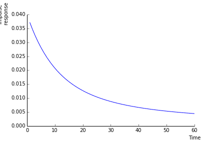
• The short term impact of a shock \(dB_{t}\) on the log price is \(\sigma\).

• As of time \(T\), the impact on the log price has become \(\sigma (1-\sigma_{\lambda}b(T-t)).\)

• In the long run, it is \(\sigma (1-\sigma_{\lambda}/\eta)\). How long is the long run depends on \(\eta\).

• There is excess volatility when \(\sigma_{\lambda}\) is positive.

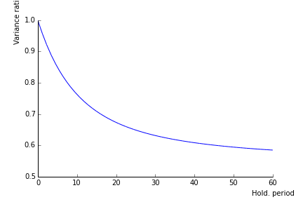
• The conditional variance of cumulated log returns over \([t,T]\) is: \[\sigma^{2}\int_{t}^{T}(1-\sigma_{\lambda}b(T-u))^{2}du,\] whereas in the case of a constant price of risk it is simply: \[\sigma^{2}(T-t).\]

• Per unit of time, we get respectively, after some lengthy calculations: \[\sigma^{2}\left[1-\frac{2\sigma_{\lambda}}{\eta}+\frac{\sigma_{\lambda}^{2}}{\eta^{2}}+(\frac{2\sigma_{\lambda}}{\eta}-\frac{\sigma_{\lambda}^{2}}{\eta^{2}})\frac{b(T-t)}{T-t}-\frac{\sigma_{\lambda}^{2}}{2\eta}\frac{b(T-t)^{2}}{T-t}\right],\] and of course: \[\sigma^{2}.\]

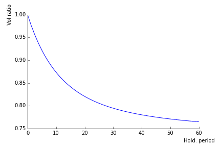
• The quantity in brackets thus describes the term structure of risk, the variance ratio.

• Here is an illustration for \(\sigma_{\lambda}=0.04\) and \(\eta=0.15.\)

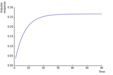
• In the graphics below, I look at a negative shock normalized to \(1\) on the price. This shock raises the price of risk by \(4\%\) immediately. The price of risk then mean reverts. The higher price of risk leads to a recovery of \(|\sigma_{\lambda}|b(\tau)\) of the price level in \(\tau\) years. This is \(\sigma_{\lambda}/\eta\) in the long run, i.e. about \(25\%\).

Investment problem

• I consider only utility of terminal wealth (horizon H), taking CRRA functions.

• The solution to HJB has the form (see Munk): \[V(t,\lambda,W)=\frac{1}{1-\gamma}\left(W e^{A_{o}(H-t)+A_{1}(H-t)\lambda+\frac{1}{2}A_{2}(H-t)\lambda^{2}}\right)^{1-\gamma}.\]

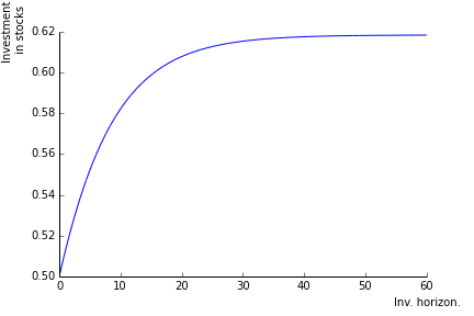
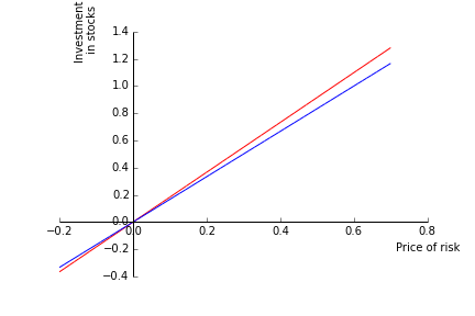
• I now look at the investment policy in this model. Computing the partial derivative, we get: \[\pi^{\star}_{t}=\frac{1}{\gamma}\frac{\lambda_{t}}{\sigma}+\frac{\gamma-1}{\gamma}\frac{\sigma_{\lambda}}{\sigma}(A_{1}(H-t)+A_{2}(H-t)\lambda).\]

• See Munk for the detailed expressions. In most cases (!) both \(A_{1}\) and \(A_{2}\) are positive implying that the hedging term is positive for risk averse investors (\(\gamma>1\)).

Data

• The data:
  • \(\sigma=20\%\)
  • \(\sigma_{\lambda}=0.04\), \(\eta=0.15\) (half life=\(4.6\))
  • \(\bar{\lambda}=0.3\)
  • \(\gamma=3\)
• With this data, the investor holds \(50\%\) in stocks \(50\%\) in cash when the price of risk is constant at \(\bar{\lambda}\)

Mean reversion and hedging properties

• Why do stocks have hedging properties?

  • I am prospectively poorer if the price of risk is low. If I hold stocks and the price of risk falls, I make profits. Indeed, a low price of risk comes through a rise in prices. Stocks thus provide insurance benefits.
  • If I engage in timing, buying when the price of risk is high and selling when the price of risk is low, I make a profit which is negative if the price of risk rises. This profits thus also has hedging properties vis-à-vis future investment opportunities. This is why the hedging term is increasing in \(\lambda\).

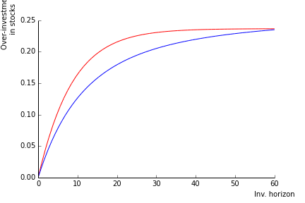
• The equity investment increases with the investment horizon, in contrast to what happens in constant investment opportunities setups (where ).

• This comes about because the hedging properties of stocks rise with investment horizon. When the investment horizon is short, there is no time to benefit from mean reversion.

• I call the volatility reduction attached to the holding period \(h\) the loss in volatility in \(\%\) experienced when holding the stock \(h\) periods. In the current calibration, the maximum reduction in vol

Links

• Link to pdf

---

1. For random vectors of any size, we have: \[\text{Cov}(X,Y)=E[XY'].\]↩︎