Dynamics, Discrete Time
Having looked at static investment problems, I now turn to dynamics starting with the discrete time case. Where static modeling is restricted to buy and hold policies, the dynamic setup allows rebalancing. Dynamic programming is introduced in a Markovian context with intermediate consumption. Some concrete problems with a terminal CRRA utility function are then solved. In the case of i.i.d. returns, the optimal policy is seen to be independent of the investment horizon, an initially counterintuitive result. It entails rebalancing to constant weights.The growth optimal portfolio which corresponds to log-utility is then considered, both when returns are i.i.d. and when they depend on a Markovian state variable. The optimal investment policy is often called the Kelly rule.
Statics versus dynamics (1)
We saw that the interpretation of the static model could accomodate distant investment horizons.
However, the portfolio is chosen at the beginning, \(t=0\) and left alone thereafter until the end of time \(t=T\). We will see that there are gains attached to changing the portfolio structure before the end of time (rebalancing gains).
We will first explore explore dynamic topics in the discrete time setup: \(t=0,1,\ldots,T\).
Static versus dynamic (2)
Wealth shares dynamics: \(\phi_{i,t+1}=\phi_{i,t}\tilde{R}_{i,t+1}=\phi_{i,t}(1+\tilde{r}_{i,t+1})\).
Portfolio shares: \[\pi_{i,t+1} =\frac{\phi_{i,t+1}}{\sum_{j\in \cal{I}}\phi_{j,t+1}}\] \[= \frac{\phi_{i,t}(1+\tilde{r}_{i,t+1})}{\sum_{j\in \cal{I}}\phi_{j,t}(1+\tilde{r}_{j,t+1})}\] \[= \frac{\pi_{i,t}(1+\tilde{r}_{i,t+1})}{\sum_{j\in \cal{I}}\pi_{j,t}(1+\tilde{r}_{j,t+1})}\] \[\approx \pi_{i,t}(1+\tilde{r}_{i,t+1}-\sum_{j\in \cal{I}}\pi_{j,t}\tilde{r}_{j,t+1}).\]
Static versus dynamic (3)
The share of the assets which outperform increase at the expense of the ones which underperform.
Over long periods of time, the buy and hold portfolio can drift significantly away from the initial portfolio and acquire unintended characteristics.
Allowing dynamic trading opens up possibilities, increasing utility outcomes.
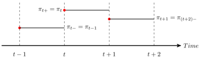
The timing sequence (1) - fig 1
- Rebalancing decisions are taken ‘right before’ each date in the discrete schedule. We assume they entail no transaction costs.
The timing sequence (2) - fig 2
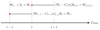
The sequential budget constraint (1)
Some changes in notation versus the static section: tildas are dropped; vectors are not denoted with bold characters any more
With consumption and income: \[W_{t+1}=Y_{t+1}+(W_{t}-C_{t})\pi_{t}'R_{t+1}.\] where:
- \(W_{t}\) is financial wealth out of which consumption is deducted to compute what’s available to financial investment
- \(Y_{t}\) is the income received in date \(t\)
Portfolio shares sum to one (\(\pi_{t}'e=1\)).
The sequential budget constraint (2)
- Without income and consumption, we get the self-financing condition (no wealth is added to or removed from the portfolio at any time): \[W_{t+1}=W_{t}\pi_{t}'R_{t+1}.\]
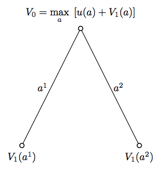
Backward induction (1) - fig 3

Backward induction (2) - fig 4

Backward induction (3) - fig 5
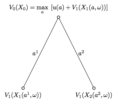
Backward induction (4) - fig 6
The state variable and the value function
At each node in the decision tree, the state variable embodies all information needed to take decisions.
In our case this means the wealth level as well as all information useful to compute the conditional distributions of future returns and income.
The value function, at each node, is the expected value of the flow of utility to be derived further down the tree, computed using the optimal controls.
Technical issues
One has to describe a proper probabilistic setup for the different stochastic processes.
In addition, we need the right convexity assumptions for the optimization program to have a unique solution described by necessary and sufficient first order conditions.
Dynamic programming (1)
We need to describe the dynamics of income and returns. As a simplification, we assume there is a scalar Markovian process \((x_{t})_{t \in [O,T]}\) such that at any date \(t\), the future distribution of income and returns is known once \(x_{t}\) is known.
Given that \((x_{t})_{t \in [O,T]}\) is Markovian, all information regarding the future state variable \(x_{t+h}\) (\(h>0\)) as of date \(t\) is summarized in the current value \(x_{t}\).
General finite horizon maximization problem: \[V_{0}(x_{0},W_{0})= \underset{(\pmb{\pi}_{[0,T]},\pmb{C}_{[0,T]})}{\text{max}} \; E_{0}[\sum_{t=0}^{T} \delta^{t}u_{t}(C_{t})]\] \[\text{s.t.}\] \[\; W_{t+1}=Y_{t+1}+(W_{t}-C_{t})\pi_{t}'R_{t+1},\] \[\pi_{t}'e=1,\] \[\; C_{t} \geq 0,\] \[\; W_{T} \geq 0.\]
Choice is over consumption and portfolio plans
Dynamic programming (2)
Solving the program entails specifying consumption and portfolio plans for all contingencies.
From a mathematical standpoint, this means that solutions are functions of the relevant state variable.
In contrast, in static problem, the optimal portfolio is a ‘constant’ (at least, given initial wealth)..
Dynamic programming (3)
We can define the value function \(V_{t}(x_{t},W_{t})\) as the solution of: \[V_{t}(x_{t},W_{t})= \underset{(\pmb{\pi}_{[t,T]},\pmb{C}_{[t,T]})}{\text{max}} \; E_{t}[\sum_{k=t}^{T} \delta^{k}u_{k}(C_{k})]\] \[\text{s.t.}\] \[\; W_{k+1}=Y_{k+1}+(W_{k}-C_{k})\pi_{k}'R_{k+1},\] \[\pi_{k}'e=1,\] \[\; C_{k} \geq 0,\] \[\; W_{T} \geq 0.\]
Value is measured as of date \(0\) here. One could instead measure value at date \(t\) as of date \(t\). For future reference, we can denote the latter \(\tilde{V}_{t}(\cdot)\). I will refer to this loosely as undiscounted value.
Dynamic programming (4)
The Bellman equation for the value function (backward induction): \[V_{t}(x_{t},W_{t})= \underset{(\pi_{t},C_{t})}{\text{max}} \; \delta^{t} u_{t}(C_{t})+E_{t}[V_{t+1}(x_{t+1},W_{t+1})]\] \[\text{s.t.}\] \[\; W_{t+1}=Y_{t+1}+(W_{t}-C_{t})\pi_{t}'R_{t+1},\] \[\pi_{t}'e=1,\] \[\; C_{t} \geq 0.\]
This equation is solved backwards
Remark: in our case, the terminal condition is known
The optimal control of the sequential problem (i.e. the problem above) is the solution of the initial intertemporal problem.
The Bellman equation is established in this post.
Written using \(\tilde{V}(\cdot)\) (undiscounted value at date \(t\)), the Bellman equation reads: \[\tilde{V}_{t}(x_{t},W_{t})= \underset{(\pi_{t},C_{t})}{\text{max}} \; u_{t}(C_{t})+\delta E_{t}[\tilde{V}_{t+1}(x_{t+1},W_{t+1})]\] \[\text{s.t.}\] \[\; W_{t+1}=Y_{t+1}+(W_{t}-C_{t})\pi_{t}'R_{t+1},\] \[\pi_{t}'e=1,\] \[\; C_{t} \geq 0.\]
Dynamic programming (5)
From the above formulation, we see that the investor will take into account the impact of the state variable on future well being.
We will see that, provided he is risk averse, he will try to protect himself against potential adverse developments (changes in \(x_{t}\)) by purchasing assets which hedge against them.
Example: the short term rate as a state variable
Dynamic programming (6)
For future reference (continuous time problems), we can write the equation followed by the value function as a difference equation: \[0= \underset{(\pi_{t},C_{t})}{\text{max}} \; \{ \delta^{t} u_{t}(C_{t})+E_{t}[\Delta V_{t+1}(x_{t+1},W_{t+1})]\}\] with: \[\Delta V_{t+1}(x_{t+1},W_{t+1})=V_{t+1}(x_{t+1},W_{t+1})-V_{t}(x_{t},W_{t}).\]
This formulation will resonate with the HJB differential equation in continuous time.
Using undiscounted value, this would read: \[0= \underset{(\pi_{t},C_{t})}{\text{max}} \; \{ u_{t}(C_{t})+E_{t}[\Delta_{\delta} \tilde{V}_{t+1}(x_{t+1},W_{t+1})]\}\] with the quasi-difference operator: \[\Delta_{\delta} \tilde{V}_{t+1}(x_{t+1},W_{t+1})=\delta \tilde{V}_{t+1}(x_{t+1},W_{t+1})-\tilde{V}_{t}(x_{t},W_{t}).\]
A first intertemporal problem (1)
In this example, we make extreme assumptions:
- i.i.d. returns: the financial opportunity set does not change over time
- no intermediate consumption: this is just a simplification
- CRRA utility: wealth accumulation does not interfere with relative risk aversion
The utility function is taken to be \(u(w)=w^{1-\rho}/(1-\rho)\) for \(\rho>1\). The case \(\rho<1\) works in a similar way. The log-utility case will be treated below.
This problem is completely solved in exercise 2.1 (see this post ).
A first intertemporal problem (2)
The problem: \[\underset{\pmb{\pi}_{[0,T-1]}}{\text{max}} \; E_{0}\left[\frac{W_{T}^{1-\rho}}{1-\rho}\right]\] \[\text{s.t.}\] \[\; W_{t+1}=W_{t}\pi_{t}'R_{t+1},\] \[\pi_{t}'e=1.\]
We will have to assume that there is a portfolio \(\pi^{0}\) such that: \[E\left[\frac{(\pi^{0}R)^{1-\rho}}{1-\rho}\right]>-\infty,\] in which case there is a solution to the one step problem that delivers finite utility.
We note that: \[E_{0}\left[\frac{W_{T}^{1-\rho}}{1-\rho}\right]=\frac{W_{0}^{1-\rho}}{1-\rho}E_{0}\left[\Pi_{t=1}^{T}(\pi^{\prime}_{t-1}R_{t})^{1-\rho}\right]\] and that therefore, the value function is homogenous of degree \(1-\rho\).
A first intertemporal problem (3)
Assume we have found the sequence of optimal portfolios \((\pi^{*}_{t})_{t=1,\cdots,T-1}\)for a given of wealth. It is then optimal for all other levels of wealth. The value function at date \(0\) is: \[V_{0}(w) =\frac{w^{1-\rho}}{1-\rho}E_{0}\left[\Pi_{t=1}^{T}(\pi^{*\prime}_{t-1}R_{t})^{1-\rho}\right]\] \[= w^{1-\rho}V_{0}(1)\]
This extends to all \(V_{t}(\cdot)\), which are seen to be proportional to \(w^{1-\rho}\)and fully determined by the constant \(V_{t}(1)\). It is important to note that \(V_{t}(1)\) is deterministic (and negative) in the present i.i.d. case.
A first intertemporal problem (4)
The optimal portfolio in each period solves: \[\underset{\pi_{t}}{\text{max}} \; E_{t}\left[V_{t+1}(1)(\pi_{t}'R)^{1-\rho}\right],\] under \(\pi_{t}'e=1.\)
The solution \(\pi^{*}\) is the same for all dates since \(V_{t+1}(1)\) drops out of the expectations.
One can easily compute \(V_{t}(1)\) by backward recursion.
A first intertemporal problem (5)
We thus have the result that in a dynamic problem where returns are i.i.d., and there is no intermediate consumption, the optimal portfolio is kept constant (through rebalancing).
The optimal portfolio is static (rebalancing).
Two features are key:
- relative risk aversion does not depend on the level of wealth
- returns are not predictable
Log utility: the value function
We now look at the log-utility case.
We have for any sequence of portfolio choices \((\pi_{t})_{t=0,\ldots,T-1}\): \[\log(W_{T}) =\log(W_{0})+\sum_{t=1}^{T} \log(\pi_{t-1}'R_{t})\] as well as: \[\log(W_{T}) =\log(W_{t})+\sum_{k=t}^{T-1} \log(\pi_{k}'R_{k+1}).\]
Assuming a state variable \(x_{t}\) characterizes the prospective returns as of date \(t\), we can write the value function as: \[V_{t}(x_{t},W_{t})=\log(W_{t})+V_{t}(x_{t},1).\]
Bellman’s equation reads: \[V_{t}(x_{t},W_{t})=\log(W_{t})+V_{t}(x_{t},1)=\underset{\pi_{t}}{\text{max}} \; E_{t}\left[\log(W_{t+1})+V_{t+1}(x_{t+1},1)\right].\] \[=\underset{\pi_{t}}{\text{max}} \; E_{t}\left[\log(W_{t})+\log(\pi_{t}'R_{t+1})+V_{t+1}(x_{t+1},1)\right].\]
Log utility: the optimal investment policy (1)
The optimal portfolio in each period therefore solves: \[\underset{\pi_{t}}{\text{max}} \; E_{t}[\log(\pi_{t}'R_{t+1})],\] under \(\pi_{t}'e=1.\)
Because the state variable drops out of the criterion to be maximized, its influence on the optimal policy \(\pi^{*}_{t}\) operates through the conditional distribution of returns. The optimal policy is determined by solving one step ahead problems as if the investment horizon at date \(t\) was not \(T\) but \(t+1\).
Log utility: the optimal investment policy (2)
- The investment policy is called myopic. In general, the investor factors in the impact of changes in the state variable on his future utility level, and accordingly, hedges adverse shocks to the state variable. Example: hedging interest rate changes…
The virtue of log utility (1)
We continue with the i.i.d. assumption
Consider an initial wealth level \(w\). Let’s compute the log of terminal wealth: \[\log(W_{T})=\log(w)+\log(W_{1})-\log(W_{0})+\cdots+\log(W_{T})-\log(W_{T-1}).\]
Using the accumulation equation \(W_{t+1}=W_{t}\pi_{t}'R_{t+1}\) and choosing a constant portfolio \(\pi\) we get: \[\frac{1}{T}\left(\log(W_{T})-\log(w)\right)=\frac{1}{T}\left(\sum_{k=1}^{T}\log(\pi'R_{t+1})\right).\]
The virtue of log utility (2)
The law of large numbers implies that for large \(T\): \[\frac{1}{T}\left(\log(W_{T})-\log(w)\right) \approx E[\log(\pi'R)].\]
As a result, a portfolio which maximizes \(E[\log(\pi'R)]\) beats any other portfolio over the long run.
This does not mean that this portfolio is optimal for finite horizon terminal wealth problems!
The virtue of log utility (3)
One can extend this result to a Markovian setup where information on future returns is summarized by a state variable \(x_{t}\).
One is led to maximize at each date: \[E_{t}\left[\log(\pi'R_{t+1})|x_{t}\right],\] which leads to a portfolio rule \(\pi^{*}(\cdot)\) that depends on the state variable.
As in the case with i.i.d. returns, the optimal growth result hinges on the law of large numbers, and the fact that the unconditional expectation can be split as follows: \[E[\log(\pi(\omega)'R(\omega))]=E[E[\log(\pi(\omega)'R(\omega))|x]].\]